Chapter 15
Introducing Correlation and Regression
IN THIS CHAPTER
 Getting a handle on correlation analysis
Understanding the many kinds of regression analysis
Correlation, regression, curve-fitting, model-building — these terms all describe a set of general statistical techniques that deal with the relationships among variables. Introductory statistics courses usually present only the simplest form of correlation and regression, equivalent to fitting a straight line to a set of data. But in the real world, correlations and regressions are seldom that simple — statistical problems may involve more than two variables, and the relationship among them can be quite complicated.
 The words correlation and regression are often used interchangeably, but they refer to two different concepts:
- Correlation refers to the strength and direction of the relationship between two variables, or among a group of variables.
- Regression refers to a set of techniques for describing how the values of a variable or a group of variables may cause, predict, or be associated with the values of another variable.
You can study correlation and regression for many years and not master all of it. In this chapter, we cover the kinds of correlation and regression most often encountered in biological research and explain the differences between them. We also explain some terminology used throughout Parts 5 and 6.
Correlation: Estimating How Strongly Two Variables Are Associated
Correlation refers to the extent to which two variables are related. In the following sections, we describe the Pearson correlation coefficient and discuss ways to analyze correlation coefficients.
Lining up the Pearson correlation coefficient
The Pearson correlation coefficient is represented by the symbol r and measures the extent to which two variables (X and Y) tend to lie along a straight line when graphed. If the variables have no relationship, r will be 0, and the points will be scattered across the graph. If the relationship is perfect the points will lie exactly along a straight line, and r will either be:
 : If the variables have a direct or positive relationship, meaning when one goes up, the other goes up, or
 : If the variables have an inverse or negative relationship, meaning when one goes up, the other goes down
Correlation coefficients can be positive (indicating upward-sloping data) or negative (indicating downward-sloping data). Figure 15-1 shows what several different values of r look like.
Note: The Pearson correlation coefficient measures the extent to which the points lie along a straight line. If your data follow a curved line, the r value may be low or zero, as shown in Figure 15-2. All three graphs in Figure 15-2 have the same amount of random scatter in the points, but they have quite different r values. Pearson r is based on a straight-line relationship and is too small (or even zero) if the relationship is nonlinear. So, you shouldn’t interpret  as evidence of lack of association or independence between two variables. It could indicate only the lack of a straight-line relationship between the two variables.

© John Wiley & Sons, Inc.
FIGURE 15-1: 100 data points, with varying degrees of correlation.

© John Wiley & Sons, Inc.
FIGURE 15-2: Pearson r is based on a straight-line relationship.
Analyzing correlation coefficients
In the following sections, we show the common kinds of statistical analyses that you can perform on correlation coefficients.
Testing whether r is statistically significantly different from zero
Before beginning your calculations for correlation coefficients, remember that the data used in a correlation — the “ingredients” to a correlation — are the values of two variables referring to the same experimental unit. An example would be measurements of height (X) and weight (Y) in a sample of individuals. Because your raw data (the X and Y values) always have random fluctuations due to either sampling error or measurement imprecision, a calculated correlation coefficient is also subject to random fluctuations.
Even when X and Y are completely independent, your calculated r value is almost never exactly zero. One way to test for a statistically significant association between X and Y is to test whether r is statistically significantly different from zero by calculating a p value from the r value (see Chapter 3 for a refresher on p values).
The correlation coefficient has a strange sampling distribution, so it is not useful for statistical testing. Instead, the quantity t can be calculated from the observed correlation coefficient r, based on N observations, by the formula 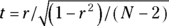 . Because t fluctuates in accordance with the Student t distribution with
  degrees of freedom (df), it is useful for statistical testing (see Chapter 11 for more about t).
For example, if  for a sample of 12 participants, then
 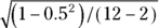 , which works out to
  , with 10 degrees of freedom. You can use the online calculator at
 https://statpages.info/pdfs.html and calculate the p by entering the t and df values. You can also do this in R by using the code:
2 * pt(q = 1.8257, df = 10, lower.tail = FALSE).
Either way, you get  , which is greater than 0.05. At α = 0.05, the r value of 0.500 is not statistically significantly different from zero (see Chapter 12 for more about α).
How precise is an r value?
You can calculate confidence limits around an observed r value using a somewhat roundabout process. The quantity z, calculated by the Fisher z transformation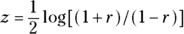 , is approximately normally distributed with a standard deviation of
  . Therefore, using the formulas for normal-based confidence intervals (see Chapter 10), you can calculate the lower and upper 95 percent confidence limits around
 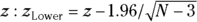 and
and 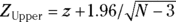 . You can turn these into the corresponding confidence limits around r by the reverse of the z transformation:
  for
for  and
and  .
.
Here are the steps for calculating 95 percent confidence limits around an observed r value of 0.05 for a sample of 12 participants (N = 12):
- Calculate the Fisher z transformation of the observed r value:
- Calculate the lower and upper 95 percent confidence limits for z:
- Calculate the lower and upper 95 percent confidence limits for r:
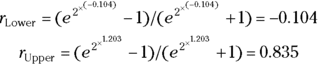
Notice that the 95 percent confidence interval goes from  to
to  , a range that includes the value zero. This means that the true r value could indeed be zero, which is consistent with the non-significant p value of 0.098 that you obtained from the significance test of r in the preceding section.
Determining whether two r values are statistically significantly different
Suppose that you have two correlation coefficients and you want to test whether they are statistically significantly different. It doesn’t matter whether the two r values are based on the same variables or are from the same group of participants. Imagine that a significance test for comparing two correlation coefficient values (which we will call  and
and  ) that were obtained from
  and
and  participants, respectively. You can utilize the Fisher z transformation to get
  and
and  . The difference (
 ) has a standard error (SE) of
  . You obtain the test statistic for the comparison by dividing the difference by its SE. You can convert this to a p value by referring to a table (or web page) of the normal distribution.
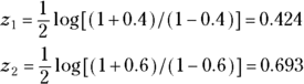
For example, if you want to compare an r1 value of 0.4 based on an N1 of 100 participants with an r2 value of 0.6 based on an N2 of 150 participants, you perform the following steps:
- Calculate the Fisher z transformation of each observed r value:
- Calculate the (
 ) difference:
- Calculate the SE of the (
 ) difference:
- Calculate the test statistic:

Look up 2.05 in a normal distribution table or web page such as
https://statpages.info/pdfs.html(or edit and run the R code provided earlier in “Testing whether r is statistically significantly different from zero”), and observe that the p value is 0.039 for a two-sided test.A two-sided test is used when you’re interested in knowing whether either r is larger than the other. The p value of 0.039 is less than 0.05, meaning that the two correlation coefficients are statistically significantly different from each other at α = 0.05.
Determining the required sample size for a correlation test
If you are planning to conduct a study where the outcome is a correlation between two variables designated X and Y, you need to be sure to enroll a large enough sample so that if the correlation is indeed statistically significant, you have enough sample for r to show it. As described in Chapter 11 with the t test and the ANOVA, the sample size can be estimated through one big equation, where you plug the estimated effect size along with the α and power you select into an equation, and calculate the sample size (see Chapter 3 for the scoop on effect size and selecting α and power).
For a sample-size calculation for a correlation coefficient, you need to plug in the following design parameters of the study into the equation:
- The desired α level of the test: The p value that’s considered significant when you’re testing the correlation coefficient (usually 0.05).
- The desired power of the test: The probability of rejecting the null hypothesis if the alternative hypothesis is true (usually set to 0.8 or 80 percent).
- The effect size of importance: The smallest r value that is considered practically important, or clinically significant. If the true r is less than this value, then you don’t care whether the test comes out significant, but if r is greater than this value, you want to get a significant result.
It may be challenging to select an effect size, and context matters. One approach would be to start by referring to Figure 15-1 to select a potential effect size, then do a sample-size calculation and see the result. If the result requires more samples than you could ever enroll, then try making the effect size a little larger and redoing the calculation until you get a more reasonable answer.
 You can use software like G*Power (see Chapter 4) to perform the sample-size calculation. If you use G*Power:
- Under Test Family, choose t-tests.
- Under Statistical Test, choose Correlation: Point Biserial model.
- Under Type of Power Analysis, choose A Priori: Compute required sample size – given α, power, and effect size.
- Under Tail(s), because either r could be greater, choose two.
- Under Effect Size, which is the expected difference between r1 and r2, enter the effect size you expect.
- Under α err prob, enter 0.05.
- Under Power (1-β err prob), enter 0.08.
- Click Calculate.
The answer will appear under Total sample size. As an example, if you enter these parameters and an effect size of 0.02, the total sample size will be 191.
Regression: Discovering the Equation that Connects the Variables
As described earlier, correlation assesses the relationship between two continuous numeric variables (as compared to categorical variables, as described in Chapter 8). This relationship can also be evaluated with regression analysis to provide more information about how these two variables are related. But perhaps more importantly, regression is not limited to continuous variables, nor is it limited to only two variables. Regression is about developing a formula that explains how all the variables in the regression are related. In the following sections, we explain the purpose of regression analysis, identify some terms and notation typically used, and describe common types of regression.
Understanding the purpose of regression analysis
You may wonder how fitting a formula to a set of data can be useful. There are actually many uses. With regression, you can
- Test for a significant association or relationship between two or more variables. The process is similar to correlation, but is more generalized to produce a unique equation or formula relating to the variables.
- Get a compact representation of your data. A well-fitting regression model succinctly summarizes the relationships between the variables in your data.
- Make precise predictions, or prognoses. With a properly fitted survival function (see Chapter 23), you can generate a customized survival curve for a newly diagnosed cancer patient based on that patient’s age, gender, weight, disease stage, tumor grade, and other factors to predict how long they will live. A bit morbid, perhaps, but you could certainly do it.
- Do mathematical manipulations easily and accurately on a fitted function that may be difficult or inaccurate to do graphically on the raw data. These include making estimates within the range of the measured values (called interpolation) as well as outside the measured values (called extrapolation, and considered risky). You may also want to smooth the data, which is described in Chapter 19.
- Obtain numerical values for the parameters that appear in the regression model formula.Chapter 19 explains how to make a regression model based on a theoretical rather than known statistical distribution (described in Chapter 3). Such a model is used to develop estimates like the ED50 of a drug, which is the dose that produces one-half the maximum effect.
Talking about terminology and mathematical notation
A regression model is a formula that describes how one variable, the dependent variable, depends on one or more other variables, and on one or more parameters. (While it is technically possible to have more than one dependent variable in a model, a discussion of this type of regression is outside the scope of this book.) The dependent variable is also called the outcome, and the other variables are called independent variables or predictors. Parameters refer to the other terms that appear in the formula that make the function come as close as possible to the observed data which are determined by the statistical software you are using.
If you have only one independent variable, it’s often designated by X, and the dependent variable is designated by Y. If you have more than one independent variable, variables are usually designated by letters toward the end of the alphabet (W, X, Y, Z). Parameters are often designated by letters toward the beginning of the alphabet (a, b, c, d). There’s no consistent rule regarding uppercase versus lowercase letters.
Sometimes a collection of predictor variables is designated by a subscripted variable ( and so on) and the corresponding coefficients by another subscripted variable (
 , and so on).
In mathematical texts, you may see a regression model with three predictors written in one of several ways, such as
 (different letters for each variable and parameter)
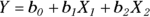 (using a general subscript-variable notation)
In practical work, using the actual names of the variables from your data and using meaningful terms for parameters is easiest to understand and least error-prone. For example, consider the equation for the first-order elimination of an injected drug from the blood,  . This form, with its short but meaningful names for the two variables, Conc (blood concentration) and Time (time after injection), and the two parameters,
  (concentration at Time
  ) and
) and  (elimination rate constant), would probably be more meaningful to a reader than
  .
.
Classifying different kinds of regression
You can classify regression on the basis of
- How many predictors or independent variables appear in the model
- The type of data of the outcome variable
- What mathematical form to which the data appear to conform
There are different terms for different types of regression. In this book, we refer to regression models with one predictor in the model as simple regression, or univariate regression. We refer to regression models with multiple predictors as multivariate regression.
In the next section, we explain how the type of outcome variable determines which regression to select, and after that, we explain how the mathematical form of the data influences the type of regression you choose.
Examining the outcome variable’s type of data
Here are the different regressions we cover in this book by type of outcome variable:
- Ordinary regression (also called linear regression) is used when the outcome is a continuous variable whose random fluctuations are governed by the normal distribution (see Chapters 16 and 17).
- Logistic regression is used when the outcome variable is a two-level or dichotomous variable whose fluctuations are governed by the binomial distribution (see Chapter 18).
- Poisson regression is used when the outcome variable is the number of occurrences of a sporadic event whose fluctuations are governed by the Poisson distribution (see Chapter 19).
- Survival regression when the outcome is a time to event, often called a survival time. Part 6 covers the entire topic of survival analysis, and Chapter 23 focuses on regression.
Figuring out what kind of function is being fitted
Another way to classify different types of regression analysis is according to whether the mathematical formula for the model is linear or nonlinear in the parameters.
In a linear function, you multiply each predictor variable by a parameter and then add these products to give the predicted value. You can also have one more parameter that isn’t multiplied by anything — it’s called the constant term or the intercept. Here are some linear functions:


In these examples, Y is the dependent variable or the outcome, and X, W, and Z are the independent variables or predictors. Also, a, b, c, and d are parameters.
The predictor variables can appear in a formula in nonlinear form, like squared or cubed, inside functions like Log and Sin, and multiplied by each other. But as long as the coefficients appear only in a linear way, the function is still considered linear in the parameters. By that, we mean each coefficient is multiplied by a term involving predictor variables, with the terms added together in a linear equation.
A nonlinear function is anything that’s not a linear function. For example:
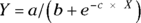
is nonlinear in the parameters, because the parameter b is in the denominator of a fraction, and the parameter c is in an exponent. The parameter a appears in a linear form, but if any of the parameters appear in a nonlinear way, the function is said to be nonlinear in the parameters. Nonlinear regressions are covered in Chapter 19.